Goals:

1. consider the relationship between macroeconomic equilibrium and full employment of resources;

2. to form students’ worldview on economic issues in general;

3. awaken interest in the subject and this topic in particular.

Keywords : consumption, savings, planned expenditures, multiplier, recessionary gap, inflationary gap

Questions:

1. Equilibrium of aggregate supply and demand and full employment of resources. Components of aggregate demand and the level of planned expenditures. Consumption and savings. Investments.

2. Actual and planned expenses. Keynes' cross. The mechanism for achieving equilibrium production volume.

3. Fluctuations in the equilibrium level of output around economic potential. Autonomous expenditure multiplier.

Question No. 1. Equilibrium of aggregate supply and demand and full employment of resources. Components of aggregate demand and the level of planned expenditures. Consumption and savings. Investments

In the world economic literature, two main directions of the mechanism for regulating national production in market conditions can be distinguished. First - the classical direction of automatic self-regulation of the market system. Its representatives are D. Ricardo, D. St. Mill, F. Edgeourt, A. Marshall, and A. Pigou. Second– Keynesian, based on the need for mandatory government intervention in the market system, especially in conditions of depression.

Classical economists assumed the flexibility of prices, wages, interest rates, i.e. from the fact that wages and prices can freely move up and down, reflecting the balance between supply and demand. In their opinion, the aggregate supply AS has the form of a vertical straight line, reflecting the potential volume of GNP production. A decrease in price entails a decrease in wages, and therefore full employment is maintained. There is no reduction in the value of real GNP. Here all products will be sold at different prices. In other words, a decrease in aggregate demand does not lead to a decrease in GNP and employment, but only to a decrease in prices. Thus, classical theory believes that government economic policy can only affect the price level, and not output and employment. Therefore, its interference in regulating production and employment is undesirable.

Classicism dominated economic science until the 30s, when the English economist D.M. Keynes published his work “The General Theory of Employment, Interest and Money.” In it, he criticized the main provisions of the classical theory, which, from his point of view, very often came into conflict with real life. Firstly, Keynes argued that the economy is not developing as smoothly, and wages and prices are not as flexible as represented in neoclassical models. Secondly, The fundamental relationships between investment, saving and interest rates were questioned. As a result, Keynes considered it impossible to achieve equilibrium automatically without government intervention. Keynes did not believe in achieving full employment by cutting wages. He believed that, despite unemployment, wages would not decrease and the labor market would remain in a disequilibrium state. Due to the existence of wage floors, there will always be a certain percentage of unemployed, and to eliminate such unemployment it is necessary to expand aggregate demand, which will cause an increase in the demand for labor.

Keynes had serious doubts about the possibility of using flexible prices. He argued that lower prices could not automatically lift an economy out of a recession and that the level of interest rates was not determined by the intersection of the saving and investment curves, but depended on the demand and supply of cash. In other words, consumers decide to save part of their income from its value and size, which determine the amount of consumption. No matter how flexible the interest rate is, it is not able to stop the decline in aggregate demand. Therefore, equilibrium can be achieved with underemployment.

When constructing the aggregate supply curve, Keynes proceeded from the assumption of a constant wage level. Since its value is constant, entrepreneurs cannot reduce production costs. This means that in this situation, price reductions are unlikely to occur.

Optimization of macroeconomic proportions is achieved through the mechanism of supply and demand. Let us consider the problem of coordinating supply and demand in relation to the owners of capital and labor.

Firms, whose administration acts as representatives of capital, produce products, earn money for it and place a demand for labor. Workers offer their labor, receive remuneration for it, and place demand for the products produced. Based on the interaction of firms and households in the market for goods and services, the proportion of GNP divided into consumption and savings is determined.

Consumption represents the individual and joint use of consumer goods aimed at satisfying the material and spiritual needs of people. In monetary terms, this is the amount of money that is spent by the population on the purchase of material goods and services. Thus, everything that is not savings, does not go as a tax, is not in foreign accounts - this is consumption. People tend to delay consumption today in the hope that consumption in the future will provide them with more utility than consumption in the present. The primary unit of consumption is the family. It determines the volume and structure of consumption. The family economy is characterized by a general consumer budget, housing and accumulated property.

Population consumption- one of the main components that determine the state of the economy.

Simplest consumption function looks like

C = a + b(Y-T),

Where WITH- consumer spending;

A - autonomous consumption, the value of which does not depend on the size of current disposable income; Kommersant - marginal propensity to consume; Y - income;

T - tax deductions;

(Y-T)- disposable income (income after tax deductions). In macroeconomic models, this indicator is often denoted as Yd or D.I.

Marginal propensity to consume- MPC)- the share of increases in spending on consumer goods and services in any change in disposable income.

Where MRS- marginal propensity to consume;

Increase in consumer spending;

average propensity to consume- ARS)- the share of disposable income that households spend on consumer goods and services.

Where ARS- average propensity to consume; C is the amount of consumer spending; Yd- amount of disposable income.

Saving- This is deferred consumption or that part of income that is not currently consumed. They are equal to the difference between income and current consumption. Saving is a process that is associated with meeting production and consumer needs in the future.

Therefore, saving is an economic process associated with investment; the part of income that remains unused when spending on current production and consumer needs accumulates. Savings are made by both firms and households. Firms save for investment - to expand production and increase profits. Households save for a number of reasons, including: providing for old age and transferring wealth to children, accumulating funds for the purchase of land, real estate and expensive durable items. Saving and investing are carried out independently of each other, by different economic entities and for different reasons.

The simplest savings function has the form:

S = -a + (1-b)(Y-T),

Where S- the amount of savings in the private sector;

A- autonomous consumption; (1 - b)- marginal propensity to save;

Y - income;

T-tax deductions.

Marginal propensity to save- MPS)- the share of the increase in savings in any change in disposable income.

Where MPS- marginal propensity to save;

Increase in savings;

Increase in disposable income.

Average propensity to save-APS)- the share of disposable income that households save.

Where APS- average propensity to save;

S is the amount of savings;

Yd- the amount of disposable income.

Household personal consumption WITH forms an essential component of effective demand. But if we remember that saving S represents the excess of income over consumer spending, then it becomes clear that when analyzing the factors that determine consumption, we simultaneously consider the factors on which saving depends.

Describing the relationship between the volume of national income and consumption expenditures, D. Keynes noted that the level of consumption depends on the level of income. “The psychology of society is such,” Keynes wrote, “that with the growth of total real income, total consumption also increases, but not to the same extent as income grows” (Keynes J. General Theory of Employment, Interest and Money. M.: Progress, 1978. P. 80). In formalized form, consumption can be expressed by the following function:

However, income is the main factor determining not only consumption, but also savings:

Research has found that consumption moves in the same direction as income. However, consumption depends not only on income, but also on the so-called marginal propensity to consume (MPC).

It is easy to see that if C+S=Y(i.e. total income is divided into consumption and savings), then . Then the sum of the marginal propensity to consume and the marginal propensity to save is equal to 1:

MRS + MPS = 1;

Investments (capital investments) on a national scale determine the process of expanded reproduction. The construction of new enterprises, the construction of residential buildings, the construction of roads, and, consequently, the creation of new jobs depend on the process of investment, or capital formation.

The source of investment is savings. But the problem is that savings are carried out by some economic agents, and investments can be carried out by completely different economic entities.

Savings of the general population are a source of investment. But these persons do not carry out capital formation associated with a real increase in capital goods. Of course, the savings of operating various firms are also a source of investment. Here the “saver” and the “investor” are the same. However, the role of savings of wage earners who are not also entrepreneurs is very significant, and the discrepancy between the processes of saving and investment due to these reasons can lead the economy to a state deviating from equilibrium.

What factors does investment depend on? Let us note the most important of them. Firstly, the investment process depends on the expected rate of return, or profitability, on the proposed investment. If this profitability, in the opinion of the investor, is too low, then the investment will be made.

Secondly, When making a decision, an investor always takes into account alternative investment opportunities, and the level of interest rate will be decisive here. An investor can invest money in the construction of a new plant or factory, or he can place his financial resources in a bank. If the rate of interest is higher than the expected rate of profit, then investments will not be made, and vice versa, if the rate of interest is lower than the expected rate of profit, entrepreneurs will carry out investment projects.

It is obvious that investment is a function of the interest rate: I = f(r) and this function is decreasing:

the higher the interest rate level, the lower the level of investment.

Savings are also a function (but already increasing) of the interest rate

It should be emphasized that such functional connections between the level of interest and the size of investments and savings were described in the works of theorists of the classical school. In the Keynesian concept of investment, just like the classics, there is a function of the interest rate, but savings, according to J. Keynes, is a function of income: S = S (Y). At this point, J. Keynes disagrees with A. Marshall, who linked the amount of savings with the interest rate.

So, investment is a function of the interest rate, and saving is a function of income. Thus, the modern Keynesian concept emphasizes that the dynamics of investment and savings are determined by various factors.

Investments depend on the level of taxation and the general tax climate in a given country. Too high a level of taxation does not stimulate investment, although the question of what tax rates should be considered high or low can hardly be resolved unambiguously.

The investment process responds to the rate of inflationary depreciation of money. In conditions of galloping inflation, when cost calculation represents significant uncertainty, the processes of real capital formation become unattractive, and preference will be given to speculative operations.

Simplest Autonomous Investment Feature has the form:

I = e - dR,

where I is investment expenses independent of total income;

e- autonomous investments determined by external economic factors (mineral reserves, etc.);

R- real interest rate;

d- empirical coefficient of investment sensitivity to interest rate dynamics.

Marginal propensity to invest- share of the increase in investment expenses in any change in income:

Where - change in the amount of investment;

Change in income.

Question 2. Actual and planned expenses. Keynes' cross. Mechanism for achieving equilibrium production volume

Actual investment include both planned, so and unplanned investments. The latter represent unanticipated changes in investment in inventories. These unplanned investments function as an equalizing mechanism that brings actual savings and investments into line and establishes macroeconomic equilibrium.

Planned expenses represent the amount that households, firms, governments, and the outside world plan to spend on goods and services. Real costs differ from planned when firms are forced to make unplanned investments in inventories in the face of unexpected changes in sales levels.

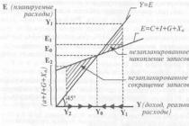
Function of planned expenses E = C + I + G + Xn depicted graphically as a function of consumption C - a + b(Y - T), which is “shifted” up by the amount I + G + X p.

Obviously, the line of planned expenses will intersect the line at which real and planned expenses are equal to each other (that is, the line Y = E), at one point A. The given drawing is called Keynes' cross. On line Y = E equality of actual investments and savings is always maintained. At the point A, where income is equal to planned expenses, equality of planned and actual investments and savings is achieved, that is, macroeconomic equilibrium.

As a result of studying this chapter, the student should:

know

• components of aggregate demand and planned expenditures;
• mechanism for achieving equilibrium production volume in the Keynesian “income-expenses” model;
• concepts of inflationary and recessionary gaps;

be able to

• determine the factors affecting the macroeconomic equilibrium in the “income-expenses” model;
• calculate indicators of average and marginal propensity to consume and save, expenditure multiplier, accelerator;

own

• skills in graphically depicting the “income-expenses” model;
• the ability to determine the factors that ensure macroeconomic balance in the “income-expenses” model;
• skills in analyzing public policy measures based on the “income-expenses” model.

Equilibrium of the commodity market in the “income-expenses” model

Another model that reflects the relationship between aggregate demand and aggregate supply is the Keynesian income-expenditure model, which is also called the Keynesian cross. It is based on the assumption of fixed prices, which differs from the AD - AS model.

Let us note the main provisions of Keynesian theory, which over the course of several decades of the 20th century. formed the basis of the macroeconomic policies of the leading countries of the world:

• It is not aggregate supply that determines demand, but aggregate demand that determines the level of economic activity, i.e. aggregate supply and employment levels;
• wages and prices are not completely flexible;
• the interest rate does not equalize the volumes of savings and investments;
• Full employment is not achieved automatically; government intervention in economic processes is necessary.

In the Keynesian model, aggregate demand depends on the consumption and saving functions. Unlike classical economic theory, according to which the main factor determining the dynamics of savings and investment is the interest rate, according to Keynes both consumption and savings are functions of income.

The factors determining the dynamics of consumption and savings include:

• household income;
• wealth accumulated by households;
• price level;
• economic expectations;
• the amount of consumer debt;
• level of taxation.

The values ​​of consumption and savings, provided that the state does not take special actions to change them, are relatively stable. Current consumption is less than the amount of income by the amount of savings. Therefore, to maintain balance it is necessary that savings were transformed into investments. It should be noted that the investment activities of business entities are very variable.

Let us list the factors that determine the dynamics of investment:

• expected rate of net profit;
• real interest rate;
• level of taxation;
• changes in production technology;
• cash fixed capital;
• economic expectations;
• dynamics of total income.

To achieve equilibrium at full employment, according to Keynesian theory, the government must stimulate aggregate demand. Therefore, this theory is often called the theory of aggregate demand. The insufficiency of aggregate demand is due to two main reasons.

1. The action of the basic psychological law, according to which, as income grows, people increase the share of income going to savings: “The psychology of society is such that with the growth of total real income, total consumption also increases, but not to the same extent as income grows.” . To describe this pattern, indicators of the average and marginal propensity to consume and save are used.

Average propensity to consume APC = C/Y shows what proportion of income goes to consumption.

Average propensity to save APS = S/Y characterizes the share of income that is saved.

Marginal propensity to consume MRS = AC/AY shows the change in consumption depending on changes in income.

Marginal propensity to save MPS = AS/AY determines the change in the amount of savings depending on changes in income.

2. Low rate of return on capital due to high interest rates (this reduces investment demand from firms).

Under these conditions, the state’s task is to compensate for the fall in aggregate demand with the help of government spending.

In the Keynesian income-expenses model, market equilibrium is achieved when total (planned) expenses AE(i.e. the amount that business entities plan to spend on the purchase of goods and services) equals total income N1(national income) - real expenses incurred by firms, and N1 = DI(disposable income). N1 = D.I. denote Y. The flow of expenditure represents aggregate demand, and the flow of income represents aggregate supply. To build a model, it is necessary to write the following equalities:

From G And Exp(demand from the state and the external market) at this stage of the study we abstract.

Hence,

We build a coordinate system (Fig. 5.1). To determine the equilibrium point, it is necessary to draw a line at an angle of 45°. All points on this line are in equilibrium: expenses equal income (AE = Y). To find the equilibrium point we need, we need to build a consumption line.

In Keynesian theory, as mentioned in the previous chapter, the main factor determining the dynamics of consumption and savings is the amount of household disposable income. The consumption function has the form

Where S a- autonomous, i.e. consumption that does not depend on changes in income (let’s say it will be equal to 100 units); MRS- marginal propensity to consume (let’s take it as 0.8); Y - disposable income (income after making tax deductions).

Rice. 5.1.

Let's build a line WITH. Let's take Y to be zero. Then WITH will be equal to S a(100). Let's give Y, for example, a value of 200 units. Then WITH= 100 + + 0.8 x200 = 260.

At the point where the consumption line intersects the 45° line, all income is consumed. At consumption values ​​above this point, part of the income goes to savings. If consumption exceeds disposable income (the area to the left of the critical point), then it is carried out partly due to previous savings.

Now you need to draw a savings line and find the point where investment equals savings. Building a savings line

Where S a - autonomous saving, S a = -S a; MPS- marginal propensity to save.

At Y = 0, this line will pass through the point (-100), since all savings will go to consumption. Where the intersection of the 45° line and the consumption function is projected onto the axis OH, savings are zero (S = 0).

Now you need to find the point of intersection of the savings line with the investment line.

Investments can be autonomous or induced (stimulated). Autonomous investments do not depend on the level of income and are determined by external circumstances (mineral reserves, foreign markets, etc.). Investments are called induced if their value increases as GDP grows, i.e. they are caused by a steady increase in demand for goods. Induced investments, superimposed on autonomous ones, enhance economic growth.

The investment function has the form

Where e + 1(f) - investments independent from total income; e - autonomous investments determined by external economic factors; /(r) - real interest rate; /(U) - induced investments.

Investment demand is quite volatile, but in our example we will make the assumption that investment demand is equal to 50 units. at all income levels. By projecting the point of intersection of the line S and lines I to a line at an angle of 45°, we will find the equilibrium point. Straight AE = WITH+ / will also pass through this point (parallel to line C).

Determining the general equilibrium point is necessary to predict economic development. If at the moment the actual Y less than equilibrium, this means that firms produce less than buyers are willing to purchase (AD > AS), and it can be assumed that the economy will expand. If the national income exceeds the equilibrium level, i.e. buyers purchase less goods than firms produce (A9 AD), inventories increase, and firms reduce production.

The equilibrium level of output fluctuates in accordance with changes in the components of total expenditure (C, I, G, Exp), Moreover, an increase in expenses causes a multiple increase in income.

The question arises: by what amount will national income change as a result of changes in spending?

Autonomous spending multiplier is the ratio of the change in the equilibrium volume of national production to the change in any component of autonomous expenditure. It shows how many times the total increase (reduction) in total income exceeds the initial increase (reduction) in autonomous expenses:

Where MULT- autonomous expenditure multiplier; A Y- change in the equilibrium volume of national production; AL - change in autonomous costs, independent of the dynamics of U.

Simple multiplier formula

Let's look at the multiplication process using a simple example.

Example. Let’s assume that the increase in autonomous investments in society was 1000 units. On the one hand, these are expenses. On the other hand, income. This money materializes in the form of labor, equipment, raw materials and other goods. The owners of these factors of production will receive an income also equal to 1000 units. At MRS = They will use 0.75 for consumption of 750 units, and for savings - 250 units. 750 units also, for some they will become expenses, and for others, income (Table 5.1).

Table 5.1

Animation process

As a result, the initial investment of 1000 units. led to an increase in national income to 4000 units. (with a multiplier equal to 1/0.25 = 4, 1000 4 = 4000).

Thus, the action of the multiplier, which repeatedly increases the consequences of changes in autonomous expenditures, is a factor that enhances government stimulation of aggregate demand. At the same time, it can increase economic instability. Therefore, the government's task is to create a system of built-in stabilizers that reduce fluctuations in business activity.

As shown above, equality between aggregate demand and aggregate supply requires equality in the volumes of savings and investment: I = S. Since investment is a function of interest, and saving is a function of income, the problem of finding their equality is very difficult.

Lack of balance between planned investments and savings can lead to two negative effects on the functioning of the economy:

• inflation gap;
• deflationary gap.

The inflation gap is a situation in the economy in which planned expenditures (E along the vertical axis) exceed the potential level of aggregate output, or planned investments exceed savings (/>5) corresponding to a situation of full employment, i.e. The supply of savings by the household sector lags behind the investment needs of firms (Figure 5.2).

Rice. 5.2.

In this situation, the population will direct most of their income to consumption, demand in the markets for goods and services will increase, which will increase the rate of price growth, i.e. will cause inflation. Thus, the economy will not be able to independently reach a state of equilibrium corresponding to the point Y 0, and the inflation gap will increase due to the multiplier effect.

To overcome the inflation gap it is necessary to restrain aggregate demand and move the equilibrium to the point E ( . The reduction in equilibrium total income should be

A recessionary (deflationary) gap is a situation in the economy in which planned expenditures are less than the potential level of aggregate output or planned investments are less than savings (/S), corresponding to a situation of full employment, i.e. The supply of savings by the household sector outpaces the investment demand of firms.

In conditions of a recessionary gap, the population will save a large part of their income, demand in the markets for goods and services will decrease, which will cause overproduction and a decrease in the price level, as well as a subsequent decline in production and layoffs of workers. The decline in employment and decline in income in the economy will continue until the multiplier effect ends. Thus, the recessionary gap will gradually narrow, the economy will independently reach a state of equilibrium corresponding to the point E b however, this will be accompanied by a decline in production and unemployment.

To overcome the effects of the recessionary gap and ensure full employment of resources, it is necessary to stimulate aggregate demand (aggregate expenditure) to the point that the equilibrium moves to the point E 2. The increment in equilibrium income will be equal to

To eliminate or reduce the recessionary gap, Keynes proposed:

• implement government policies of income redistribution to increase consumer demand;
• reduce the real interest rate to increase investment demand;
• increase government spending.

To eliminate or reduce the inflation gap by reducing the components of planned aggregate expenditure (aggregate demand), Keynes proposed increasing taxes and reducing government spending.

It should be noted that the principle of animation has a two-way effect. An increase in savings by the population in conditions of underemployment and insufficient demand gives rise to the “paradox of thrift” - it reduces savings and investments in society as a whole. Even a small reduction in investment has the opposite multiplying effect - a multiple reduction in national income is due to the fact that an increase in savings at the macro level (increase MPS) may hinder economic growth. Indeed, the Keynesian cross shows that an increase in savings and, accordingly, a reduction in consumer spending reduces the equilibrium level of GDP. The mechanism of this phenomenon is simple: a reduction in consumption will cause warehouses to become overstocked with unsold goods, a reduction in the income of entrepreneurs will lead to a curtailment of investment and a reduction in production.

However, the growth of savings can also play a positive role in the economy, but only if the money market quickly and sufficiently fully transforms them into investments - then there will be no general reduction in total spending, and the structure of the economy will change in the direction of increasing the rate of accumulation, which can lead to accelerated economic growth.

• Keynes J. M. General theory of employment, interest and money. Anthology of economic classics. M.: 1993. T. 2. P. 155.

9.1. Relationship between AD-AS and IS-LM models. Major changes
nal and equations of the IS-LM model. Output of IS and LM curves. On
clone and shift of IS and LM curves. Equilibrium in the IS-LM model.

9.2. Relative efficiency of fiscal and financial
monetary policy.

9.3. Deriving the aggregate demand curve. Economic policy
in the AD-AS and IS-LM models with changes in the price level.

Relationship between AD-AS and IS-LM models. Basic variables and equations of the IS-LM model. Output of IS and LM curves. Slope and shift of IS and LM curves. Equilibrium in the IS-LM model

In the AD-AS model and the Keynesian cross model, the market interest rate is an external (exogenous) variable and is set in the money market relatively independently of the equilibrium of the goods market. The main goal of economic analysis using the IS-LM model is to combine the commodity and money markets into a single system. As a result, the market interest rate turns into an internal (endogenous) variable, and its equilibrium value reflects the dynamics of economic processes occurring not only in the money market, but also in the commodity market.

Model IS-LM(investment - savings, liquidity preference - money) - a model of commodity-money equilibrium, which allows us to identify the economic factors that determine the aggregate demand function. The model allows us to find such combinations of market interest rates R and income Y, in which equilibrium is simultaneously achieved in the commodity and money markets. Therefore, the IS-LM model is a specification of the AD-AS model.

Chapter 9. Macroeconomic equilibrium on goods 181

Basic equations of the IS-LM model:

1) Y: =C+I+G+X n - basic macroeconomic identity;

2) C=a+b(Y-T) - consumption function, where T=T a +tY;

3) I=e-dR - investment function;

4) X n =g-m"-Y-n-R - net export function;

5)M/P = k Y - h R- money demand function.

Internal model variables: Y (income), WITH(consumption), I (investment), Xn(net exports), R(interest rate).

External model variables:G(government spending), ms(offer of money) t(tax rate).

Empirical coefficients(a, b, e, d, g, t", p, k, h) positive and relatively stable.

In the short term, when the economy is not in a state of full employment of resources (Y=Y*), price level R is fixed (predetermined), and the interest rate is R and total income Y are mobile. Because the P = const, insofar as the nominal and real values ​​of all variables coincide.

In the long term, when the economy is at full employment of resources (Y=Y*), price level R mobile In this case the variable ms(money supply) is a nominal value, and all other variables in the model are real.

IS curve- equilibrium curve in the commodity market. It represents the locus of points characterizing all combinations Y And R, which simultaneously satisfy the income identity, consumption, investment and net export functions. At all points of the IS curve, investment and savings are equal. The term IS reflects this equality (Investment = Savings).

The simplest graphical derivation of the IS curve involves the use of the saving and investment functions (see Figure 9.1).

In Fig. 9.1,A shows the savings function: with increasing income from y 1 to Y 2 savings increase with S 1 to S 2 .

In Fig. 9.1,V shows the investment function: an increase in savings reduces the interest rate from R 1 to R 2 and increases investment from I 1 to I 2 . At the same time I 1 = S 1 , a I 2 = S 2 .

In Fig. 9.1,C The IS curve is shown: the lower the interest rate, the higher the level of income.

182 Macroeconomics

A. Savings function

Similar conclusions can be drawn With using the Keynesian cross model (see Fig. 9.2).

On Fig. 9.2, A shows the investment function: an increase in the interest rate from R] before ri reduces planned investments from I(Rj) before I(Rj.

In Fig. 9.2,V Keynes's cross is depicted: a decrease in planned investment reduces income from Y/ to Y? .

In Fig. 9.2, C shows the IS curve: the higher the interest rate, the lower the level of income.

Chapter 9. Macroeconomic equilibrium on goods 183

and money markets. Model IS-LS

Algebraic derivation of the IS curve

The IS curve equation can be obtained by substituting Equations 2, 3 and 4 into the basic macroeconomic identity and solving it for R and Y.

184 Macroeconomics

The coefficient characterizes angle of inclination of the curve

howl IS relative to the axis Y, which is one of the parameters of the comparative effectiveness of fiscal and monetary policies.

The IS curve is flatter provided that:

1) investment sensitivity (d) and net exports ( n)
to the dynamics of interest rates is high;

2) marginal propensity to consume (b) big;

3) the marginal tax rate (t) is low;

4) the marginal propensity to import (m") is small.

Driven by increased government spending G or tax cuts T the IS curve shifts to the right. A change in tax rates / also changes the angle of its inclination. In the long run, the slope of IS can also be changed by income policy, since high-income families have a relatively lower marginal propensity to consume than low-income families. Other parameters (d, n And T") are practically not affected by macroeconomic policy and are predominantly external factors that determine its effectiveness.

LM curve- equilibrium curve in the money market. It records all combinations Y And R, which satisfy the demand function for money at the value of money supply set by the Central Bank M s. At all points on the LM curve, the demand for money is equal to its supply. Term L.M. reflects this equality (Liquidity Preference = Money Supply) (see Fig. 9.3).

Chapter 9. Macroeconomic equilibrium on goods 185

and money markets. Model IS-LS

Rice. 9.3,A shows the money market: growth in income from y 1 before y 2 increases the demand for money and therefore increases the interest rate R 1 to R 2 Rice. 9.3,V shows the LM curve: the higher the level of income, the higher the interest rate.

1. CONDITION FOR JOINT EQUILIBRIUM OF COMMODITY AND MONEY MARKETS 3 The goal is a more in-depth analysis of the interaction between the real sector of the economy (commodity markets) and the money market. Commodity markets will mean not only markets for consumer goods and services, but also the market for investment goods, which are not fundamentally different from consumer goods. Although there are some differences between these categories of goods, they are due only to the demand for them, since the demand for consumer and investment goods depends on different variables.

1. CONDITION FOR JOINT EQUILIBRIUM OF COMMODITY AND MONEY MARKETS 4 The demand for consumer goods is associated mainly with income, while for investment goods it is primarily with the interest rate. A distinction of this kind is superficial, since in order to significantly distinguish between the markets for consumer and investment goods, it is necessary to know their relative prices. Since the Keynesian model does not do this, economists combine markets for all goods into one market.

1. CONDITION FOR JOINT EQUILIBRIUM OF COMMODITY AND MONEY MARKETS 5 The money market is a mechanism for the purchase and sale of short-term credit instruments such as treasury bills and commercial paper. This market should be distinguished from the bond market. The relative price of money expressed in terms of bonds is the interest rate on the bonds. The challenge is to accurately define the functioning of each of these markets and, more importantly, to identify the relationships between them.

1. CONDITION FOR JOINT EQUILIBRIUM OF COMMODITY AND MONEY MARKETS 6 When considering the AD-AS model, this relationship was assumed, because changes in the prices of goods and services directly affect the demand for money. In turn, fluctuations in the interest rate in the money market are reflected in the amount of total expenses, primarily consumption and investment. In the IS-LM model (investment savings preference liquidity money), the commodity and money markets will appear as sectors of a single macroeconomic system. The model determines the equilibrium values ​​of the interest rate i and income level Y depending on the conditions prevailing in these sectors of the economy.

1. CONDITION FOR JOINT EQUILIBRIUM OF COMMODITY AND MONEY MARKETS 7 The IS-LM model was first proposed in 1937 by J. Hicks (“Hicks cross”) as an interpretation of the essence of the macroeconomic concept of J. Keynes and therefore is a specification of the AD-AS model. It became widespread after the publication of A. Hansen’s book “Monetary Theory and Fiscal Policy” in 1949, after which it also began to be called the Hicks Hansen model.

1. CONDITION FOR JOINT EQUILIBRIUM OF COMMODITY AND MONEY MARKETS 8 The IS curve reflects the relationship between the interest rate / and the level of national income Y, at which equilibrium is ensured in the commodity market. The condition for such equilibrium is the equality of the volumes of aggregate demand and aggregate supply. In this case, demand (in the absence of the state and abroad) acts as the sum of demand for consumer and investment goods. Knowing that investment is a negative function of the interest rate, and consumption is a positive function of real income, we can write the aggregate demand equation as follows: AD= C(Y)+I(i)

1. CONDITION FOR JOINT EQUILIBRIUM OF COMMODITY AND MONEY MARKETS 9 As for the supply, in accordance with the Keynesian interpretation it has the form: AS = C(Y) + S(Y) It follows that the equilibrium state in the commodity market can only take place when observing the following equality: I(i) = S(Y) This equation, established by J. Keynes, differs from the equilibrium condition on the product market in the classic model: I(i) - S(i). The only difference between them is the difference in the arguments of the savings function. This difference means that in the classical model the equilibrium between investments and savings has a unique solution, since it is achieved by itself in the market for borrowed funds at the intersection point of curves I and S

1. CONDITION FOR JOINT EQUILIBRIUM OF COMMODITY AND MONEY MARKETS 10 In the Keynesian model, a plurality of equilibrium states in the commodity market is allowed: the IS curve, which is a set of multiple equilibrium points corresponding to each pair of values ​​of the interest rate i and national income Y, acts as the equilibrium curve of the commodity market. All points of the IS curve are points of equality of savings and investments at different values ​​of the interest rate and national income. Thus, the IS curve does not reflect the functional relationship between the interest rate and income, but a set of equilibrium situations in the goods market, which are obtained as a result of the projection of the saving function and the investment function.

1. CONDITION FOR JOINT EQUILIBRIUM OF COMMODITY AND MONEY MARKETS 11 The IS curve has a negative slope, since a decrease in the interest rate increases the volume of investment, and therefore aggregate demand, thereby increasing the equilibrium value of income. The IS curve may shift when factors other than the interest rate change. Such factors include the level of consumer spending, the level of government purchases, net taxes, changes in investment volumes at the existing interest rate (as a result of a shift in the curve, i.e., an increase in investment demand I d)

Go). This will lead to an increase in the equilibrium volume of production and income (Y1 " title=" Fig. 1. Shift of the IS curve when government spending changes. Suppose, as a result of targeted actions of the state, the volume of government spending increases (G, > Go). This will lead to an increase in the equilibrium volume of production and income (Y1" class="link_thumb"> 12 !} Rice. 1. Shift of the IS curve when government spending changes Suppose that as a result of targeted government actions, the volume of government spending increases (G, > Go). This will lead to an increase in the equilibrium volume of production and income (Y1 > Yo). At the same interest rate, the equilibrium amount of income will be greater than before. Curve IS 0 will shift to the right, to position IS 1 1. CONDITION FOR COLLECTIVE EQUILIBRIUM OF COMMODITY AND MONEY MARKETS 12 Go). This will lead to an increase in the equilibrium volume of production and income (Y1 "> Go). This will lead to an increase in the equilibrium volume of production and income (Y1 > Yo). At the same interest rate, the equilibrium volume of income will be greater than before. The IS 0 curve will shift to the right, to position IS 1 1. CONDITION FOR JOINT EQUILIBRIUM OF COMMODITY AND MONEY MARKETS 12"> Go). This will lead to an increase in the equilibrium volume of production and income (Y1 " title=" Fig. 1. Shift of the IS curve when government spending changes. Suppose, as a result of targeted actions of the state, the volume of government spending increases (G, > Go). This will lead to an increase in the equilibrium volume of production and income (Y1"> title="Rice. 1. Shift of the IS curve when government spending changes Suppose that as a result of targeted government actions, the volume of government spending increases (G, > Go). This will lead to an increase in the equilibrium volume of production and income (Y1"> !}

Rice. 2. Shift of the IS curve when investment demand changes. A similar effect will be observed when the investment plans of entrepreneurs change (increasing optimism or pessimism at any interest rate), which will lead to a shift in the investment demand curve Id, and therefore to a shift in the line of total expenditures, followed by the IS curve will also shift 1. CONDITION FOR JOINT EQUILIBRIUM OF COMMODITY AND MONEY MARKETS 13

1. CONDITION FOR JOINT EQUILIBRIUM OF COMMODITY AND MONEY MARKETS 14 Now let us turn to the money market. The LM curve has been shown to reflect the relationship between interest rate i and income level Y that arises in the money market. Each point of the LM curve means the equality of the demand for money L and the supply of money M s. Such equilibrium in the money market is achieved only if, with an increase in income Y, the interest rate i will increase. To delve deeper into this condition, recall that in the Keynesian theory of the demand for money, three motives are distinguished: transactional, precautionary and speculative. The first two motives reflect the traditional role of money as a means of circulation and payment, therefore in the economic literature they are usually combined under the general concept of transaction demand, which depends on the level of disposable income: Lt = L(Y).

1. CONDITION FOR JOINT EQUILIBRIUM OF COMMODITY AND MONEY MARKETS 15 Speculative demand for money is demand from assets, and it depends on the interest rate: at a low rate, economic agents give preference to liquidity (store wealth in the form of cash), on the contrary, at a high interest rate prefer to store wealth in securities. Therefore, speculative demand for money is a decreasing function of the interest rate: La = L(i).

1. CONDITION FOR JOINT EQUILIBRIUM OF COMMODITY AND MONEY MARKETS 16 J. Keynes’s identification of speculative demand for money is an important element of his theory of effective demand. Keeping savings in liquid form reduces overall effective demand, since money as property is not spent on personal consumption and is not converted into investment. Savings, existing in the form of securities, are essentially loan capital. Therefore, they increase both consumer and investment demand. Consequently, when the speculative demand for money increases, effective demand ceases, and vice versa. The total demand for money consists of the demand for money for transactions and speculative demand and is, respectively, a function of income and interest rate: L=L(Y,i) Thus, equilibrium in the money market presupposes the fulfillment of the following condition: Ms=L(Y ,i)

1. CONDITION FOR JOINT EQUILIBRIUM OF COMMODITY AND MONEY MARKETS 17 Fig. 3. The influence of changes in income on the demand for money and the interest rate with a fixed supply of money. At a given level of income, the equilibrium of the money market will be at the point of intersection of the Lo curve with the money supply line Ms, as shown in Fig. 3,a. If the level of income changes, for example, upward (Fig. 3, a), this will lead to an increase in the demand for money (a shift of the Lo curve to position L1) and an increase in the interest rate from i 0 to i 1

1. CONDITION FOR JOINT EQUILIBRIUM OF COMMODITY AND MONEY MARKETS 18 Fig. 3. The influence of changes in income on the demand for money and the interest rate with a fixed supply of money. As a result, we obtain a set of equilibrium situations at the points of intersection of supply lines with the demand curves for money L 0, L 1, etc. This means that for each paired value of the interest rate rates and income will correspond to their equilibrium state of the money market. Graphically, the money market equilibrium line will be represented by the LM curve as a positive function of the interest rate and national income.

1. CONDITION FOR JOINT EQUILIBRIUM OF COMMODITY AND MONEY MARKETS 19 Fig. 3. The influence of changes in income on the demand for money and the interest rate with a fixed supply of money Figure 8-3, b shows that an increase in income from Y 0 to Y 1 increases the demand for money (shift L 0 to position L 1) and, therefore , increases the interest rate from i 0 to i 1,. In Fig. Figure 3b shows the LM curve, illustrating an important condition for the equilibrium of the money market: as income increases, the interest rate must rise.

1. CONDITION FOR JOINT EQUILIBRIUM OF COMMODITY AND MONEY MARKETS 20 Curve The LM curve has a specific configuration: horizontal and vertical parts. The horizontal part of the LM curve reflects the fact that the interest rate cannot fall below the minimum value i min, and the vertical part of this curve shows that beyond the maximum level of the interest rate i max, no one will hold savings in liquid (monetary) form, and will turn them into securities. A shift in the LM curve will occur when the money supply changes or the price level changes.

1. CONDITION FOR JOINT EQUILIBRIUM OF COMMODITY AND MONEY MARKETS 21 Fig. 4. Equilibrium in the IS-LM model A joint equilibrium of the commodity and money markets is achieved at the point of intersection of the IS and LM curves (Fig. 4). The IS-LM model also makes it possible to find combinations of the market interest rate and the level of income (output), at which equilibrium is simultaneously achieved in the commodity and money markets.

1. CONDITION FOR JOINT EQUILIBRIUM OF COMMODITY AND MONEY MARKETS 22 The IS and LM curves are constructed not only for a given price level P, but also for given levels of government spending G, tax revenue T and money supply M. In this case, there is only one combination of interest rate values and the level of income (iE, YF) at which equilibrium is achieved simultaneously in the two markets under consideration. The intersection of the IS and LM curves at point E means that the money supply is sufficient for an interest rate that balances planned investment and saving. Since the IS curve is related to planned expenditures, its changes reflect changes in fiscal policy. The LM curve reflects changes in monetary policy as it relates to the money supply. Thus, the IS-LM model allows us to assess the joint impact of fiscal (fiscal) and monetary (monetary) policies on the macroeconomy.

1. CONDITION FOR JOINT EQUILIBRIUM OF COMMODITY AND MONEY MARKETS 23 Fig. 5. Changes in equilibrium in a system of two markets In Fig. Figure 5a shows the change in equilibrium in the system of two markets with a decrease in the price level P (provided that the values ​​of G, T and M remain unchanged). In this case, the IS curve does not change its position, since when the price level P on the goods market decreases, the main factors that determine its configuration (government expenditures, taxes, and expected income) remain the same. The LM 0 curve will shift to the right (LM 1) because the real money supply M/P will increase in this case.

1. CONDITION FOR JOINT EQUILIBRIUM OF COMMODITY AND MONEY MARKETS 24 Consequently, equilibrium in the system of commodity and money markets can be achieved at a lower interest rate i, and a higher level of output Y 1 compared to the initial position of the curve LM 0. Thus, the equilibrium shifts from point E o to point E 1. Since the price level has decreased (which is equivalent to an increase in the real supply of money M/P), then, with constant values ​​of G, T and M, the volume of aggregate demand in the goods market will increase. The result of this change is shown in Fig. 5, b, which shows the aggregate demand curve AD, reflecting the relationship between the price level and volumes of purchases of goods and services. This is a downward-sloping curve because lower prices correspond to more cash balances. The amount of aggregate demand in the goods market, corresponding to the joint equilibrium in the goods and money markets, is called effective demand.

Macroeconomic equilibrium in the goods market (IS model)

Model IS (investment - savings) is a theoretical equilibrium model of only commodity markets with fixed prices. It reflects the relationship between the interest rate ( r) and the value of national income ( Y), which is determined by Keynesian equality.

In the analysis presented by J.M. Keynes and the Stockholm School of Economics, aggregate demand equals the demand for consumer and investment goods:

And aggregate supply is equal to national income ( Y), which is used for consumption and savings:

Equilibrium in commodity markets for the entire economy will look like: or, from here:

That is, savings and investments depend, respectively, on income levels and interest rates.

The resulting Keynesian equilibrium condition allows for multiple equilibrium states of commodity markets, since interest rate and income conditions in the economy can constantly change.

To determine this set of equilibrium states of commodity markets, the English economist John Hicks used the investment-savings model ( IS). This model allows us to find in each specific case the relationship between the interest rate ( r) and national income ( Y), at which investment is equal to savings, other factors being constant.

Model IS is considered in the short term, when the economy is not in a state of full employment of resources, the price level is fixed, the value of total income ( Y) and interest rates ( r) are mobile.

“Investment-savings” model - IS has great practical significance, since it can be used to show how much the interest rate needs to be changed when national income changes in order to maintain equilibrium in commodity markets. For example, if the interest rate is reduced, investment will increase, which will lead to an increase in planned spending and an increase in national income. In turn, an increase in national income will cause an increase in savings in society and vice versa.

Rice. 3

macroeconomic equilibrium commodity market

If we depict these processes graphically, we get a decreasing curve IS(Fig. 3).

Curve IS- this is the locus of points characterizing all combinations Y And r, which simultaneously satisfy the identity of income to the functions of consumption, saving and investment.

Curve IS divides the economic space into two areas: at all points lying above the curve IS the supply of goods exceeds the demand for them, i.e., the volume of national income is greater than planned expenses (stocks accumulate in society). At all points below the curve IS there is a shortage in the commodity market (society lives on debt, inventories are declining).

Investments are inversely related to the rate of interest. For example, with a low interest rate, investments will grow. Income will increase accordingly Y and savings will increase slightly S, and the interest rate will decrease to stimulate the conversion S V I. Hence the slope of the curve shown in (Fig. 3) IS.

This is explained by the fact that in the first case, at a higher interest rate and a certain level of income, people prefer not to consume, but to put money in the bank, i.e. save, which reduces investment and aggregate demand. In the second case, at a low interest rate, society lives in debt and prefers consumption, thereby increasing investment in the economy and its total costs.

If you change factors that were previously considered unchanged, for example, government spending ( G) or taxes ( T), then the curve IS will shift up to the right or down to the left depending on changes in the named indicators.

For example, if government spending increases and taxes remain unchanged during an expansionary fiscal policy, then the curve IS move up to the right. If taxes increase and government spending remains at the same level while implementing a contractionary fiscal policy, then the curve IS will move down to the left.

So the model IS can be and is used in business practice to illustrate the impact of state fiscal policy on national income.

Curve IS- equilibrium curve in the commodity market. It represents the locus of points characterizing all combinations Y And R, which simultaneously satisfy the income identity, consumption, investment and net export functions. At all points of the curve IS equality of investment and savings is maintained. Term IS reflects this equality ( Investment=Savings).

The simplest graphical output of a curve IS associated with the use of savings and investment functions (see Fig. 2).